Automated PCB Component Detection & Pick-and-Place

End-to-End Pipeline

From raw camera frame to physically sorted component — every step is automated.

1

Capture

4K camera with 3× digital zoom, CLAHE contrast enhancement, Laplacian sharpness selection (best of 30 frames)

→

2

Detect

YOLO11 Large Segmentation identifies components with pixel-level masks; centroid computed via image moments

→

3

Transform

Degree-3 polynomial maps pixel coordinates to printer millimeters, with phase-correlation drift compensation

→

4

Probe

Two-speed BLTouch probing measures Z height of each component (1mm fast chunks, 0.1mm precision chunks)

→

5

Pick & Place

Vacuum nozzle picks up component at (X, Y, Z), travels to the correct drop bin, releases and scrapes

YOLO11 Model Architecture

380 layers, 132.7 GFLOPs, trained on an NVIDIA A100 GPU

Backbone

Layers 0–9

Extracts features at multiple scales from the raw 1024×1024 input image.

Conv + SiLU blocks with stride 2 halve spatial dimensions: 1024 → 512 → 256 → 128 → 64
C3k2 blocks (CSP Bottleneck) with skip connections for gradient flow
SPPELAN — multi-scale spatial pyramid pooling (5×5, 9×9, 13×13 kernels)

Neck (FPN + PAN)

Layers 10–22

Fuses features across scales so the model can detect both tiny resistors and large ICs.

FPN (top-down) sends semantic info to high-res layers via upsample + concat
PAN (bottom-up) sends spatial detail to deep layers via stride-2 conv + concat
Outputs 3 feature maps: P3 (256×256), P4 (128×128), P5 (64×64)

Segment Head

Layer 23

Predicts bounding boxes, class probabilities, and instance segmentation masks simultaneously.

86,016 prediction cells across the 3 feature maps
32 mask coefficients per detection × 32 shared prototype masks
Final mask = sigmoid(coeffs × prototypes) — ProtoNet architecture

Input 1024 × 1024 × 3

↓

Backbone C3k2 + Conv + SPPELAN 1024→512→256→128→64 spatial | 3→64→128→256→512 channels

↓

P5 64²

P4 128²

P3 256²

↓

Neck (FPN + PAN) Multi-scale feature fusion

↓

Segment Head Boxes + Classes + 32 Mask Coefficients + 32 Prototype Masks (ProtoNet)

↓

NMS → Final Detections + Masks

Training Process

4 datasets, 48+ raw class labels unified into 20 classes

FPIC

Supervisely

6,260 images

Bitmap + polygon masks, 25 raw classes

Dataset Ninja PCB

Supervisely

1,299 images

Polygon annotations, 9 raw classes

WACV 2019

PASCAL VOC

47 boards

XML bounding boxes, 19 raw classes

Roboflow E-Caps

YOLO Detection

+additional

Bounding boxes → converted to 4-corner polygons

Class Unification

48+ raw labels merged into 20 unified classes. Examples:

C, cap1–cap4, capacitor → SMD Capacitor

R, CR, resistor, resestor → Resistor

U, IC, ic → IC

Q, QA, transistor → Transistor

FB, ferrite, emi → Ferrite Bead

mov, Mov, MOV, V → Varistor

Connector Diode Electrolytic Capacitor Ferrite Bead Fuse IC Inductor Jumper LED MOSFET Module Potentiometer Resistor Resistor Network SMD Capacitor Switch Test Point Transformer Transistor Varistor

Training Metrics

Loss Functions

CIoU Box Loss w = 7.5

Complete Intersection over Union. Penalizes center distance, overlap, and aspect ratio mismatch. Highest weight because pickup accuracy depends directly on box precision.

Segmentation Loss w = 1.0

Binary Cross-Entropy + Dice Loss on predicted masks vs. ground-truth masks. Dice directly optimizes global overlap to handle background pixel imbalance.

Classification BCE w = 0.5

Per-class binary cross-entropy. Lowest weight because classification is the easiest sub-task once localization is learned.

Distribution Focal Loss w = 1.5

Predicts a probability distribution over box coordinates instead of a single value. Handles ambiguous component boundaries gracefully.

Key Hyperparameters

Image Size	`1024 × 1024`	High resolution for small SMD components
Batch Size	`10` (auto)	Fills 60% of A100 80GB VRAM
Optimizer	`AdamW`	Adaptive LR with decoupled weight decay
Learning Rate	`0.001 → 0.00001`	Cosine annealing schedule
Warmup	`3 epochs`	Prevents gradient explosion at start
Early Stopping	`patience=20`	Stops if no improvement for 20 epochs
Mosaic	`1.0`	4 images stitched per sample; off last 10 epochs
Transfer Learning	`COCO pretrained`	1071/1077 layers transferred
Oversampling	`2×–5×`	Classes below 1000 instances duplicated
Mixed Precision	`AMP (FP16)`	~2× training speed on A100

Camera → Printer Coordinate Transform

Degree-3 polynomial fit mapping pixels to millimeters

The Problem

The camera sees pixels. The printer moves in millimeters. The camera is mounted at an angle, and the wide-angle lens introduces barrel distortion. A simple linear scaling fails.

The Solution

A degree-3 polynomial with 10 feature terms per axis, fit via least-squares regression on 10+ manually calibrated reference points.

Feature vector for pixel (x, y): [1, x, y, x², xy, y², x³, x²y, xy², y³] Transform: printer_X = c\cdotfeatures printer_Y = d\cdotfeatures Solved with np.linalg.lstsq(A, dst)

Why Not Homography?

A 3×3 homography assumes a perfect pinhole camera and a single plane. It cannot model the nonlinear barrel distortion from the wide-angle lens. The cubic polynomial terms (x³, y³, x²y, xy²) capture these distortions.

1

Place visible mark on printer bed

2

Jog nozzle over mark, record printer X,Y

3

Click mark in camera image, record pixel X,Y

4

Repeat 10+ times across entire work area

5

Fit polynomial via least squares regression

Drift Compensation

Phase correlation in the frequency domain (FFT) detects sub-pixel camera drift between the calibration reference frame and the current frame. The offset is subtracted before the polynomial transform.

(dx, dy), confidence = cv2.phaseCorrelate(ref, cur)

Hardware System

Modified 3D printer + Arduino + BLTouch + vacuum gripper

How the Nozzle Becomes a Gripper

A standard 3D printer has a hotend nozzle and a heated bed — neither of which are useful for picking up components. The key modification is a custom toolhead mounted alongside the original hotend on a stepper-driven rail:

The original hotend nozzle and heated bed are not used for printing. The printer is repurposed purely as a precision XYZ gantry.
A vacuum nozzle (thin tube connected to a vacuum pump) is mounted on the toolhead. When the pump turns on, suction grips the component from above.
A TMC5160 stepper motor on a rail switches between three tool positions: LEFT (camera clear), MIDDLE (BLTouch probe), and RIGHT (vacuum nozzle aligned for pickup).
The BLTouch probe measures exact Z height of each component so the vacuum nozzle knows precisely how far to descend. Without this, the nozzle would either miss the component or crash into the board.

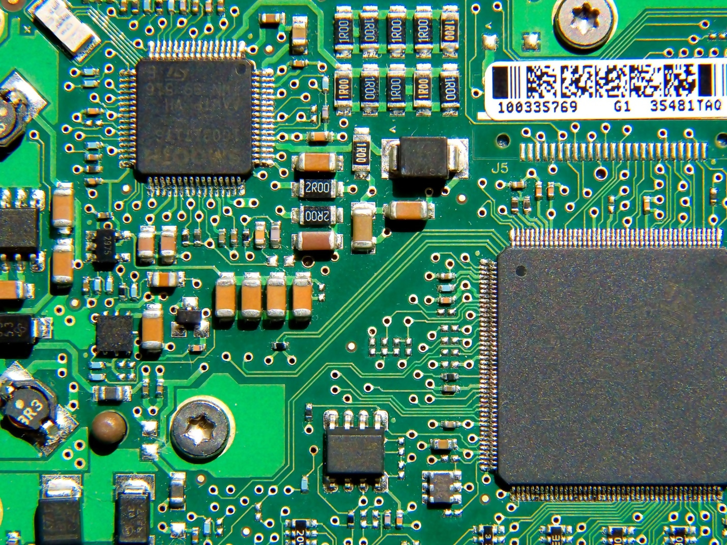
The heated bed stays off — the PCB sits flat on the unheated bed surface, held in place by its own weight. The bed provides a flat, known reference plane for the coordinate system.

Stepper Rail (TMC5160)

LEFT Camera clear

MIDDLE BLTouch probe

RIGHT Vacuum nozzle

PCB on unheated bed

Klipper 3D Printer

WebSocket / Moonraker API

Repurposed as a precision XYZ gantry (no printing)
JSON-RPC 2.0 over WebSocket for real-time command/response
Position query via printer.objects.query
Safe Z = 130mm, probing lower bound = 90mm
1.5× feedrate when ascending (no collision risk)

Vacuum Pickup System

Arduino relay + vacuum pump

Vacuum nozzle: thin tube that grips components via suction
Pump controlled by digital relay — ON to pick, OFF to release
Nozzle descends to BLTouch-measured Z height + offset
1-second dwell time ensures secure grip before raising
Scrape sequence after release dislodges any stuck components

Arduino Controller

Serial 115200 baud

TMC5160 stepper (SPI): switches tool positions on rail
16× microstepping, 3200 steps/rev, 400mA RMS
BLTouch probe: servo deploy/retract, rising-edge trigger
Two modes: stepper vs. BLTouch (mutual exclusion for safety)
Error monitoring: overtemp, short-to-ground, open load every 1s

Two-Speed Probing

BLTouch + Klipper coordinated

Fast phase: Z > 115mm — 1mm chunks @ 6000 mm/min
Slow phase: Z ≤ 115mm — 0.1mm chunks @ 150 mm/min
Arduino checks trigger after each chunk completes
On trigger: record Z, immediately raise 10mm
Probe-to-nozzle offset: X=9.2, Y=7.5, Z=−17.5 mm

Pick & Place Workflow

1 Initialize: connect Arduino + Klipper, home stepper to MIDDLE

2 Camera detects components → pixel centroids → polynomial transform to mm

3 BLTouch probes each component (capacitors first, then ICs) to get Z height

4 Switch stepper to RIGHT — moves vacuum nozzle into pickup position above the board

5 Move to component XY → vacuum ON → lower to probed Z → wait 1s for grip → raise to safe Z

6 Travel to drop bin (capacitors: bin A, ICs: bin B) → vacuum OFF → scrape nozzle to release

7 Repeat for all detected components, then park stepper and disconnect

Results

84.5% Box mAP@50

Average precision across all 20 component classes at 50% IoU threshold

84.0% Mask mAP@50

Instance segmentation accuracy — masks track closely with box accuracy

69.1% Box mAP@50-95

Strict metric averaged over IoU thresholds from 50% to 95%

<1mm Pickup Accuracy

Sub-millimeter coordinate transform + 0.1mm Z probing resolution

Epoch-by-Epoch Training

Epoch	Box Loss	Seg Loss	Cls Loss	Box mAP50	Mask mAP50
1	1.302	1.604	1.747	44.2%	43.8%
5	1.061	1.216	0.990	65.8%	65.6%
10	0.936	1.074	0.739	76.2%	76.0%
15	0.877	1.008	0.632	81.4%	80.9%
20	0.843	0.963	0.575	83.5%	82.9%
24	0.811	0.941	0.529	84.5%	84.0%

Real Model Output

Actual YOLO11 inference on a PCB image at conf=0.25 — 116 detections across 19 classes

Input Image

Model Output (116 detections)

All Detections (sorted by confidence)

Technology Stack

ML Framework
Ultralytics YOLO11 + PyTorch

Computer Vision
OpenCV 4.8+

GPU
NVIDIA A100 80GB (training)

Firmware
Klipper + Moonraker

Microcontroller
Arduino + TMC5160

Language
Python 3.12 + C++ (Arduino)

Automated PCB ComponentDetection & Pick-and-Place